
Paper Notes - PaliGemma: A versatile 3B VLM for transfer

Intro
Gemma is an autoregressive decoder-only open LLM that comes in 2B and 7B variants, both pretrained and instruction fine-tuned. PaliGemma combines the 400M SigLIP and 2B Gemma model into a sub-3B VLM that maintains performance comparable to PaLI-X, PaLM-E, and PaLI-3.
Model
PaliGemma takes as input one or more images, and a textual description of the task (the prompt or question, which is referred to as the prefix). PaliGemma then autoregressively generates a prediction in the form of a text string (i.e. the answer, which is referred to as the suffix).
Architecture
Image encoder: shape-optimized ViT-So400m image encoder that was contrastively pretrained at large scale via the sigmoid loss
Decoder-only language model: Gemma-2B
Linear projection: A linear layer projecting SigLIP’s output tokens into the same dimensions as Gemma 2B’s vocab tokens, so they can be concatenated
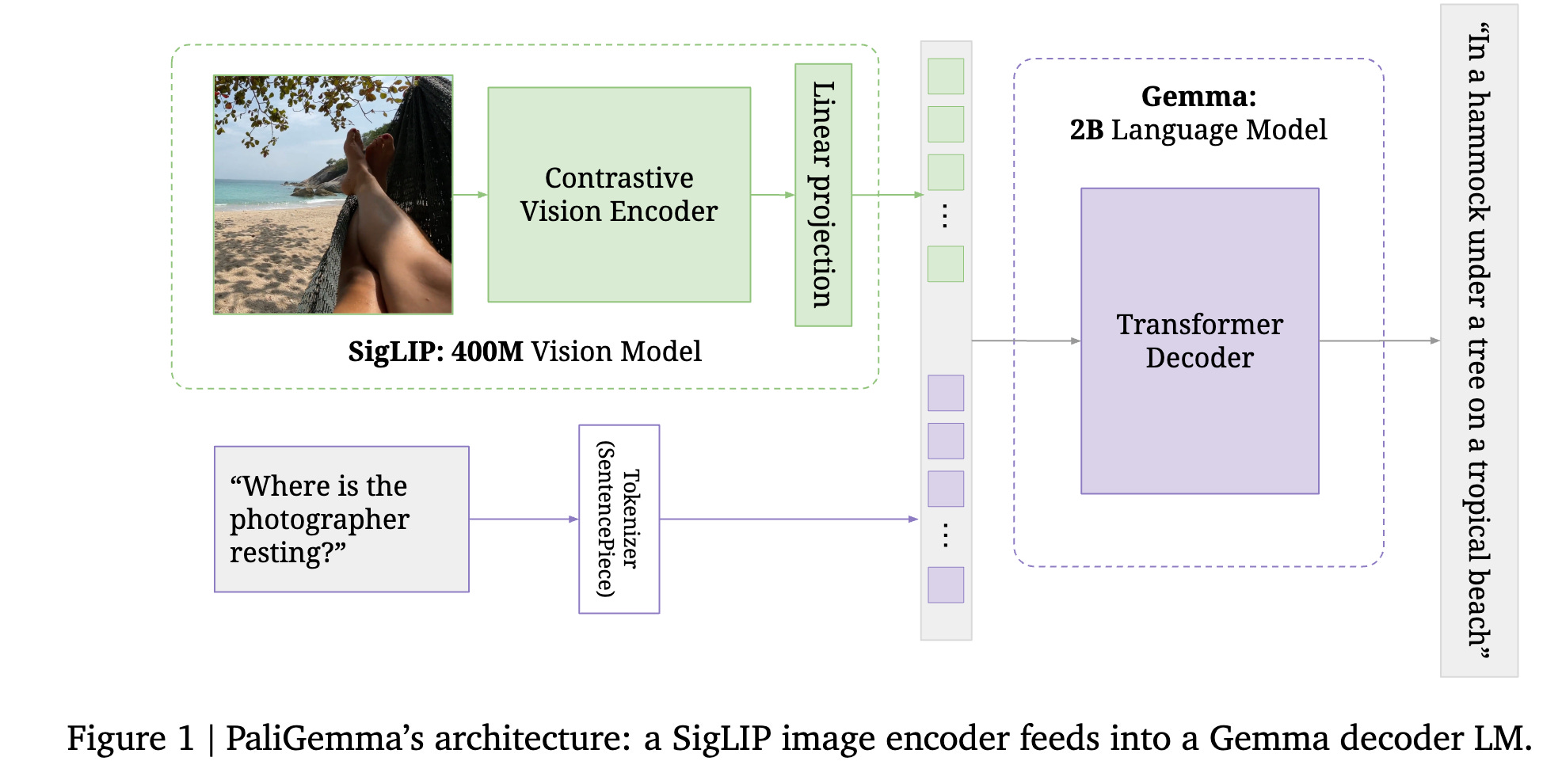
The image is passed through the image encoder, which turns it into a sequence of N_img tokens. The text is converted into N_txt tokens, using Gemma’s SentencePiece tokenizer, and embedded with Gemma’s vocabulary embedding layer. The image tokens are projected with the (zero initialized) linear projection. The sequence of input tokens to the decoder is created as follows:
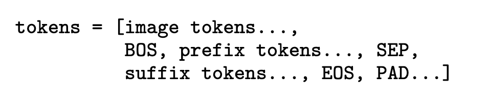
The image is always resized to a fixed square size (256, 1024, or 4096 tokens) depending on the model variant. This makes image tokens straightforward to interpret without the need for special location markers. The BOS token marks the start of text tokens and \n is used as the SEP token as it does not appear in any of the prefixes. SEP is also tokenized separately to prevent it from being merged with the prefix or suffix.
They apply full (unmasked) attention on the whole input, i.e. the image and prefix tokens. In this way, image tokens can also lookahead at the task at hand (prefix) in order to update their representation.
Pretraining
Training happens in 4 stages: unimodal pretraining (using off the shelf components), multimodal pretraining (long pretraining on a carefully chosen mixture of multimodal tasks—nothing is frozen), resolution increase (short continued pretraining at higher resolution), and transfer (turns the base model into a task-specific specialist).
Stage 1: Multimodal pretraining
Common practice suggests that the image encoder should be frozen during the first multimodal pretraining stage. This is partly due to findings reporting multimodal tuning of pretrained image encoders degrading their representations. However, more recent work has shown that captioning and other harder-to-learn tasks can provide valuable signal to image encoders, allowing them to learn spatial and relational understanding capabilities which contrastive models like CLIP or SigLIP typically lack.
Thus, in the interest of learning more skills during pretraining, PaliGemma also does not freeze the image encoder. However, to avoid destructive supervision signal from the initially unaligned language model, they use a slow linear warm-up for the image encoder’s learning-rate, which ensures that the image encoder’s quality is not deteriorated from the initially misaligned gradients coming through the LLM.
Stage 1 is trained at a resolution of 224px (hence N_img = 256) and sequence length N_txt = 128 for a total of 1 billion examples.
Stage 2: Resolution increase
The model resulting from stage 1 is already quite useful for many tasks but it can only understand images at 224x224 pixels. Hence, they train two further model checkpoints for increased resolution, first to 448x448 for 50M examples and then to 896x896 for 10M examples.
For simplicity, stage 2 consists of the exact same mixture of tasks and datasets as stage 1, but with significantly increased sampling of tasks that require high resolution. Additionally, these upweighted tasks all can be modified to provide much longer suffix sequence lengths. For example, for OCR tasks, they request the model to read all text on the image in left-to-right, top-to-bottom order and for detection/segmentation tasks, they request the model to detect or segment all objects for which annotation is provided. To do this, they increase the text sequence length to N_txt = 512 tokens.
Stage 3: Transfer
After pretraining, PaliGemma requires fine-tuning to adapt to specific tasks. The base models, trained at resolutions of 224px, 448px, and 896px, are not optimized for user-friendly or benchmark-ready use. Transfer learning is applied to refine the model for specialized tasks such as COCO Captions, Remote Sensing VQA, Video Captioning, and InfographicQA. Fine-tuning modifies all model parameters, with key hyperparameters like resolution, learning rate, label smoothing, and dropout explored per task. The model also supports multi-image tasks, where each image is encoded separately, and fine-tuning with multiple images involves concatenating the image tokens.
Pretraining task mixture
PaliGemma’s pretraining aims for strong transferability rather than zero-shot usability. The model is exposed to a diverse set of vision-language tasks to develop broad capabilities. Tasks are prefixed uniquely to prevent conflicting learning signals. No transfer datasets are included in pretraining, and near-duplicates of evaluation task images are removed. The pretraining dataset includes captioning (in 100+ languages), OCR, visual question answering, object detection, segmentation, and grounded captioning. Unlike some models, PaliGemma does not rely on GPT-4-generated instruction-following data.
Ablations
Key takeaways:
Multimodal pretraining duration
Shorter pretraining generally hurts, and skipping stage 1 entirely is terrible. However, there is a lot of variation among tasks, which highlights the need for a broad and diverse set of evaluation tasks.
Causal masking and learning objective
Extending the autoregressive mask to the prefix tokens and the image tokens hurts performance compared to the prefix-LM setting.
If you apply the next-token prediction loss on the
prefix(once it is autoregressively masked), the performance is worse than if you just applied it on thesuffix(output) only. The hypothesis was that applying it on the prefix could provide more learning signal to the model by asking it to guess the question, but the experiments show that it reduces average performance.Using task-prefixes in pretraining helps the model distinguish between different tasks, reducing uncertainty when the task is not explicitly clear. While this has minimal impact on performance after transfer, pretraining validation perplexities show that tasks with clear instructions, like VQA, do not benefit, whereas more ambiguous tasks see noticeable improvements in prediction confidence.
Overall, they find that the prefix-LM with task-prefix and supervision only on the suffix tokens is an effective VLM pretraining objective.
New token initialization
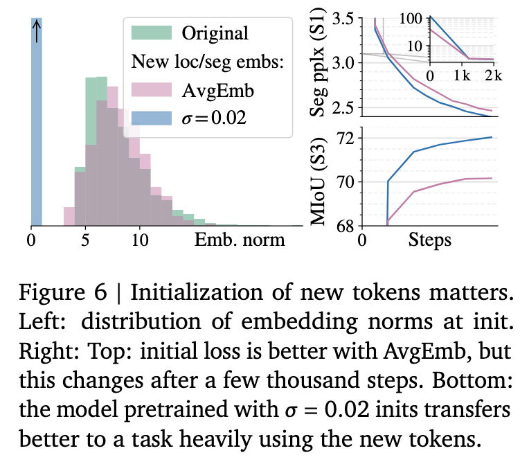
In order to add support for PaliGemma to perform more structured computer vision tasks (like detection, referring expression, and grounded captioning), they add 1024 location tokens (<loc0000> to <loc1023>), which correspond to binned normalized image coordinates. They also add 128 VQVAE tokenized single-object mask tokens (<seg000> to <seg127>) to support referring expression segmentation.
The question then is, given that all other vocabulary tokens have already been trained as part of Gemma’s pre-training, how do you initialize the embeddings of these tokens? They compare two strategies. The first is to use a standard small Gaussian noise initialization. The second, championed by some previous works, argues for matching the average of the pre-trained embeddings plus small noise. They compare these strategies and find that while the AvgEmb strategy significantly improves initial perplexity of tasks using the new tokens, this gain vanishes after a thousand steps of training. Instead, the standard initialization strategy results in significantly better Stage 1 perplexities at the end of pretraining, and also results in significantly better transfer of the model to tasks using these tokens.
To freeze or not to freeze?
Not freezing any part of the model is better during pretraining and significantly improves the validation perplexity of tasks requiring spatial understanding.
Connector design
They compare using a linear connector versus an MLP connector to map SigLIP output embeddings to the inputs of Gemma. The linear connector is just a single linear layer, whereas the MLP connector is formed of one hidden layer with GeLU non-linearity. They also explore two Stage 1 pretraining settings: tune all weights or freeze everything but the connector.
They found that there was no performance difference between the linear and MLP connector in the case of tuning all the weights, but in the all-frozen scenario, the MLP connector performed worse than the linear (69.7 vs. 70.7). Thus, their conclusion is that the linear connector is preferable (presumably because it works just as well while being smaller).
Image encoder
They investigate whether a dedicated SigLIP image encoder is necessary for good performance or whether a simplified “decoder-only” approach—where raw image patches are linearly projected and fed directly into the language model—can suffice. The authors note that nearly all VLMs use an image encoder (for example, CLIP, SigLIP, or VQGAN) to convert an image into “soft tokens” before handing it off to the language model. In contrast, only a couple of works (Fuyu and EVE) have experimented with removing the image encoder entirely.
In their ablation, the authors replace the SigLIP encoder with a simple linear projection of the raw RGB patches. Although this Fuyu‐style architecture still produces a unified decoder-only model, its performance significantly lags behind the default model that uses the pre-trained SigLIP encoder. A key factor is sample efficiency: the SigLIP encoder has been pretrained in Stage 0 on a vast dataset (approximately 40 billion image–text pairs), which gives it a strong visual prior. In the alternative setup, images are introduced for the first time during Stage 1 and the model sees only up to 1 billion examples. Despite the poorer overall performance, the authors observe that the model’s performance does improve with longer pretraining, hinting that with sufficient training data the simpler architecture might eventually catch up.
Image Resolution
PaliGemma provides three separate checkpoints at resolutions of 224px, 448px, and 896px.
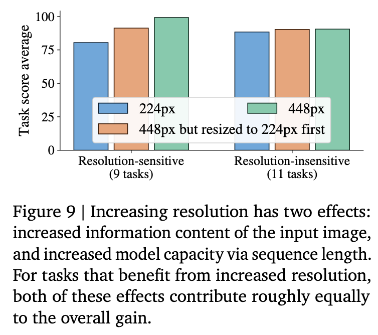
Resolution or sequence length?
Typically you get either neutral or improved performance across tasks when increasing the resolution of the input image. However, it is unclear whether this improvement comes from the fact that the image has higher resolution and therefore more information, or whether it is thanks to the resulting longer sequence length and thus increased model FLOPs and capacity. They disentangle these by running Stage 2 and transfers at 448px resolution, but downscaling each image to 224px before resizing it to 448px. Thus, the model gets to see the information content of a low-res image but with the model capacity of the high-res setting. Figure 9 shows that for those tasks for which resolution has an effect at all, the reason for the improved performance is split roughly equally between these two causes.
Need resolution specific-checkpoints?
The authors compare using a checkpoint trained at one resolution on inputs at a different resolution. Their findings show that a checkpoint natively trained at a particular resolution (for example, 448 px) performs significantly worse when applied to images at another resolution (such as 224 px), even when the higher-resolution model benefits from additional pretraining. This mismatch highlights the importance of having dedicated checkpoints for each resolution, ensuring that the model is optimally adapted to the specific details and token representations associated with each resolution level.
Thus, in the absence of flexible-resolution modelling tricks such as FlexViT or NaViT, they recommend running extended pretraining for increasing resolution (Stage 2) and providing separate checkpoints for all supported resolutions.
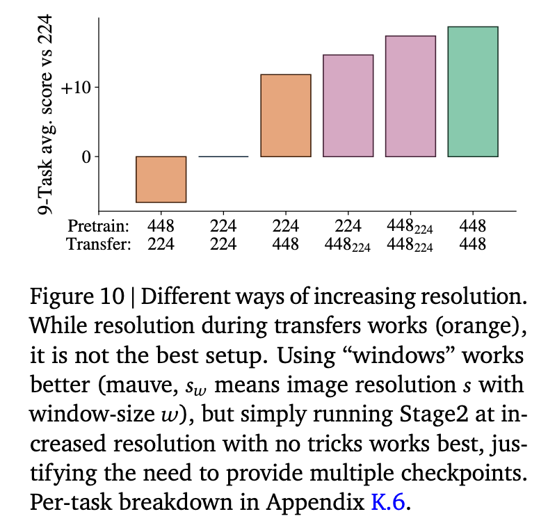
To resize or to window?
Rather than simply resizing a high-resolution image down to a lower resolution, an alternative explored is windowing. In this approach, a high-resolution image is segmented into several fixed-size windows that are individually processed by the vision encoder before their outputs are concatenated. While windowing helps preserve more visual detail than straightforward downsampling, experiments show that its performance still falls short of that achieved by training the model natively at the higher resolution. Moreover, any speed gains from windowing are modest since the main computational load remains with the language model component.
Mixture Re-weighting in High-Resolution Training
During high-resolution pretraining, the authors experiment with adjusting the sampling ratios of tasks that particularly benefit from higher resolutions. They compare this re-weighted mixture against using the same task ratios as in the low-resolution stage. While the unadjusted mixture slightly degrades performance on a few tasks (e.g. DocVQA, ChartQA, XM3600), the overall differences remain within per-task variance. This suggests that although re-weighting can offer minor improvements, it is not critical for achieving strong transfer performance.
Transferability
Repeatability
Experiments reveal that both the pretraining and transfer stages exhibit high repeatability. When the model is retrained with different random seeds, the final performance metrics show minimal variation—typically within 1–2%. This consistency confirms that the training process is robust and that the model's transfer capabilities are reliably reproducible across runs.
Transfer hyper-parameter sensitivity
The authors assess the impact of using a unified, simplified set of hyper-parameters compared to extensive per-task tuning. Their results demonstrate that the performance differences are relatively minor. This low sensitivity indicates that PaliGemma can be effectively transferred to a variety of tasks with minimal hyper-parameter tuning, simplifying its practical deployment.
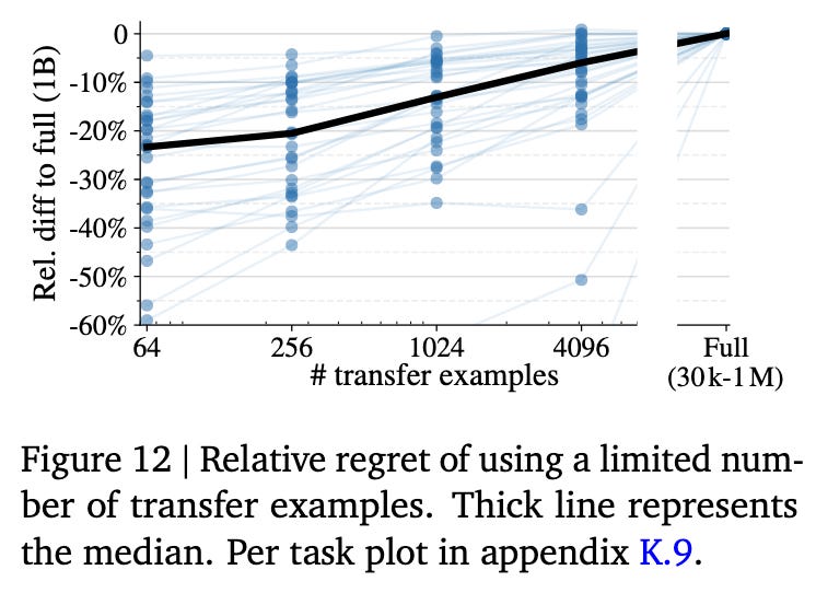
Transfer with Limited Examples
The authors evaluate how few examples are needed to effectively adapt the model to a new task by fine-tuning it with subsets of 64, 256, 1024, and 4096 examples. The findings reveal that even with as few as 64 examples, the model can achieve results that are often close to those obtained with full datasets—typically within 10–20% of the full-data performance. This demonstrates that PaliGemma is sample-efficient and capable of rapid adaptation in low-resource scenarios, despite some inherent variance in outcomes when training on very limited data.
Noteworthy Tidbits
A few additional insights emerged during the course of this work. For instance, the authors found that simply resizing images to a square format is as effective for segmentation tasks as using more elaborate aspect-ratio preserving and cropping augmentations. They also introduce CountBenchQA to overcome limitations in existing counting benchmarks, addressing issues like skewed distributions and noisy labels. Furthermore, they discovered that previously reported WidgetCaps numbers contain evaluation inconsistencies, and that providing image annotations directly via a red box yields similar results to using explicit location tokens in the prompt. Other observations include that RoPE interpolation during upscaling does not offer any benefits, and impressively, the model generalizes well to 3D renders in a zero-shot setting. Lastly, their results on the MMVP task are notably strong, outperforming several competitive models by a substantial margin.